Secondary operations

Note

Data availability for this tutorial: the medium sized data set of 614 genes and 48 taxa that will be used can be downloaded here.

In addition to one of the main operations of TriFusion (Conversion, Concatenation and Reverse concatenation), one or more secondary operations can be applied during the processing of alignment files.

How main and secondary operations interact

Before starting with the secondary operations that are available on TriFusion, it is worth clarifying how the main and secondary operations interact:

• Conversion: Each secondary operation is applied independently on each active input alignment that will be converted.
• Concatenation: With the exception of the Filter secondary operation, all remaining secondary operation are performed on the single concatenated alignment file.
• Reverse concatenation: Secondary operations will be applied after the reverse concatenation, which means that they will be applied to each partition (output file) that will be generated. It’s similar to the Conversion operation.

The order of operations

For performance reasons, operations in TriFusion are executed in a specific order:

1. Reverse concatenation [main]
2. Filters [secondary]
3. Concatenation [main]
4. Collapse [secondary]
5. Gap coding [secondary]
6. Consensus [secondary]
7. Write to file

Ok, so let’s start with the tutorial.

Load data

As already covered in a separate tutorial (see Load data into TriFusion), alignment data can be loaded into TriFusion in three different ways. Here we will use the file browser to load an entire directory where 614 alignments files are stored.

Navigate to Menu -> Open/View Data and click the Open file(s) button. This will open the main file browser.

The input data type is already correctly set to Alignment/Sequence set, so we’ll leave that as it is. Then, navigate the file browser until you find the directory containing the alignment files. In this case, all alignments are stored in a directory named Version2. Since TriFusion supports the selection of directories (in which case all files inside the specified directory will be loaded), I will only select the Version2 directory and click Load & go back button. At the end of the data loading, a popup informs how many files were loaded.

Note

If you know that not all files in the selected directory are alignments, you could still load that particular directory. All invalid alignment files will be ignored when the data is loaded.

You’ll also need to check the general options that are common to all operations.

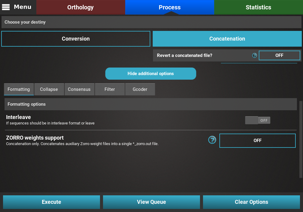
Displaying secondary operations

To display all secondary operations, click the Show additional options button. This will reveal a tabbed panel, where the secondary operations are sorted into categories (with the exception of the Formatting tab, which is not a secondary operation per se).

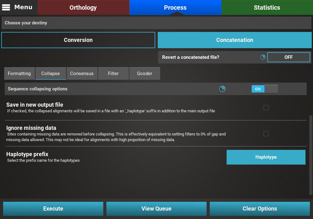
Collapse

Turn the collapse switch ON to activate the operation.

The Collapse secondary operation contains three options:

• Save in new output file: This will save the collapse alignment in another output file, separated from the main concatenated/converted output file. Checking this option will effectively produce two output files - a main output that is only concatenated/converted and another output file with the suffix “_collapsed” that will be concatenaded AND collapses. For now, we will not check this option.
• Ignore missing data: If this option is checked, sequences will be collapsed based on alignment columns that do not contain missing data and the output alignment will also contain 0% of missing data. The currently loaded data set has a fair amount of missing data, and is most likely not appropriate for collapsing using this option, so we will also leave this unchecked.
• Haplotype prefix: Sets the prefix for the haplotypes that will appear as the taxa names in the output file. An auxiliary file with the suffix “_haplotypes” will also be generated when performing this operation matching the new haplotype prefix to the original taxon names. Here we can change the default value to anything, like Haplotype

Note

You can click the Execute button to execute the Collapse operation alone, or combine other secondary operations before.

Consensus

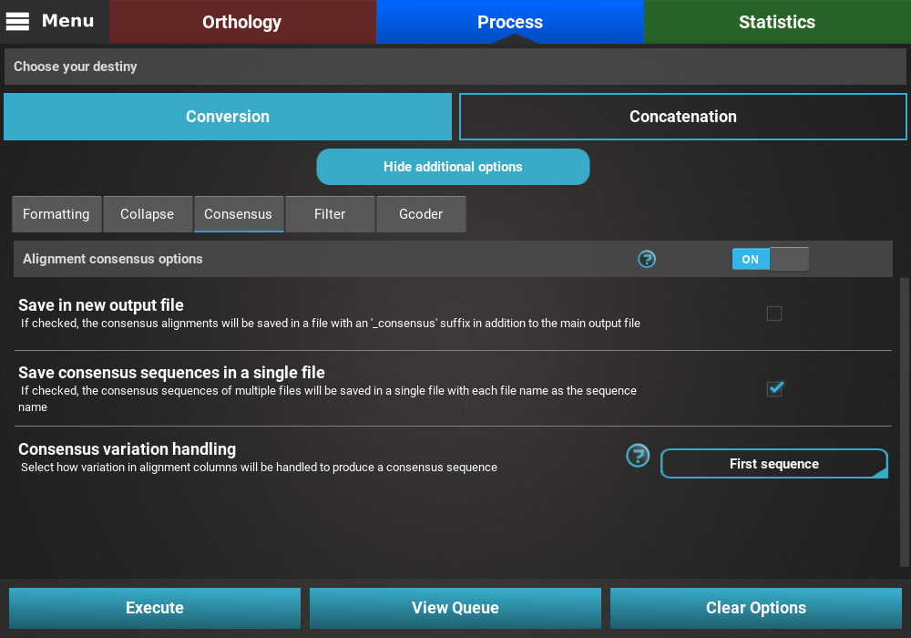
Turn the consensus switch ON to activate the operation.

The consensus operation is mainly used to compress multiple sequences in an alignment into one representative sequence. While it can be done on top of the Concatenation main operation, what this will do is concatenate all 614 alignments into a single concatenated one and then create a consensus of that large alignment. However, in the majority of the cases, users are more interested in creating a consensus sequence for each input alignment. With this in mind, this secondary operation should be done with the Conversion main operation.

The Consensus secondary operation contains three options:

• Save in new output file: This will save the consensus alignment in another output file, separated from the main concatenated/converted output file. Checking this option will effectively produce two output files - a main output that is only concatenated/converted and another output file with the suffix “_consensus” that have the consensus performed. For now, we will not check this option.
• Save consensus in a single file: This option can be checked to merge all consensus from each input alignment in a single file. In this case, if this option is left unchecked, 614 output files will be created using this option, each with a single representative consensus sequence of the corresponding alignment. However, here we are more interested in merging all consensus sequences in a single file that will be later provided for functional annotation analyses. So we’ll check this option.
• Consensus variation handing: Select how you would like to handle variation within each alignment. The appropriate choice is highly dependent on subsequent analyses. In our case, since we want to create a dataset for Blast2GO and our alignment data is fairly variable, we’ll select the First sequence value, where the first sequence of each alignment is selected as a representative.

Note

You can click the Execute button to execute the Consensus operation alone, or combine other secondary operations before.

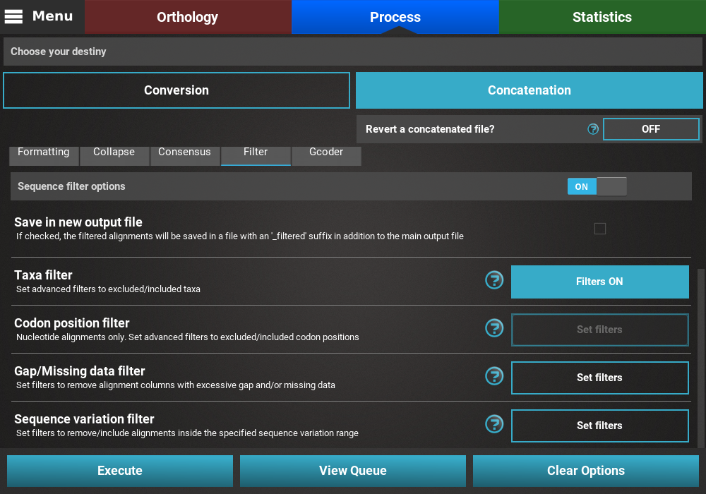
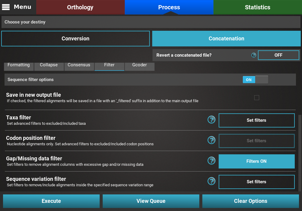
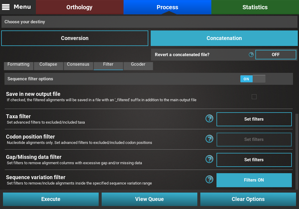
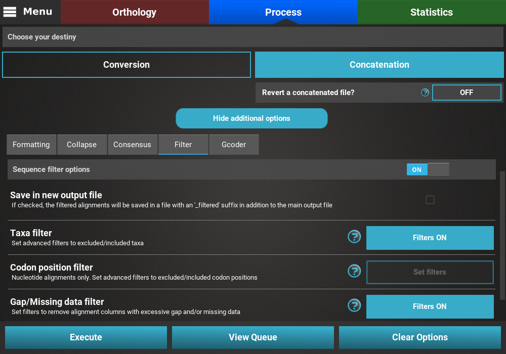
Filters

There are several Filter operations that can be applied to the alignments. Turn the filter main switch ON to activate the operation. Now you can specify one or more filters to execute in the same run. Whenever a particular filter is active, the button of the corresponding operation will display Filters set.

Note

The Codon filter operation can only be executed on nucleotide alignments, so it will be disabled when protein alignments are loaded. You can use the small 7 alignment data set for this tutorial.

Taxa filter

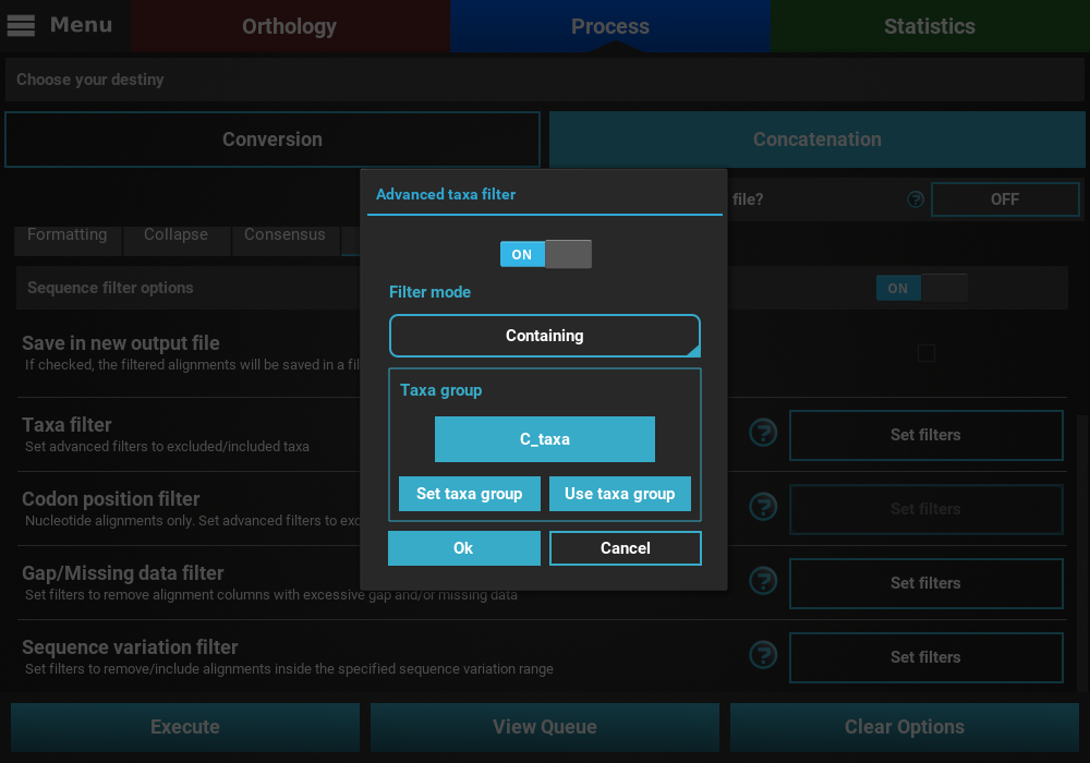
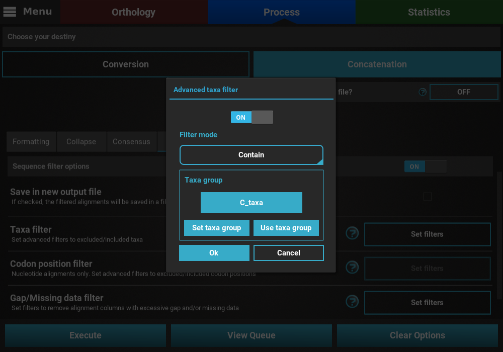
Click on the button of the Taxa filter option and turn the switch on the popup of this operation ON.

The Taxa filter operation allows users to filter entire alignments if they contain or exclude a given set of taxa. Here, we will create a fictional case where we are interested in concatenating only alignments that contain at least all taxa with names beginning on a “C”.

The filter mode sets whether the alignments should be filtered if they contain or exclude the taxa group. By default, it is set to Containing, so we’ll leave that unchanged.

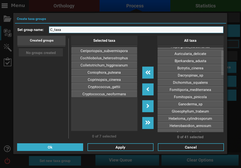
As you can see, there are no taxa groups yet defined so we’ll need to create a new one. Click the Set taxa group button to start the data set group creation process and then click the Set manually button. Here, select the desired taxa with names starting with the letter “C” and save the taxa group by clicking Ok.

Once the group has been created, it will be automatically selected in the Taxa filter dialog. Additional groups can be created in the same way. When multiple groups have been defined, they can be selected by clicking the Use taxa group button, and then selecting the desired group.

When you are happy with the Taxa filter settings, click the Ok button. If the Taxa filter switch was turned ON, the button of the Taxa filter option should change to Filters ON.

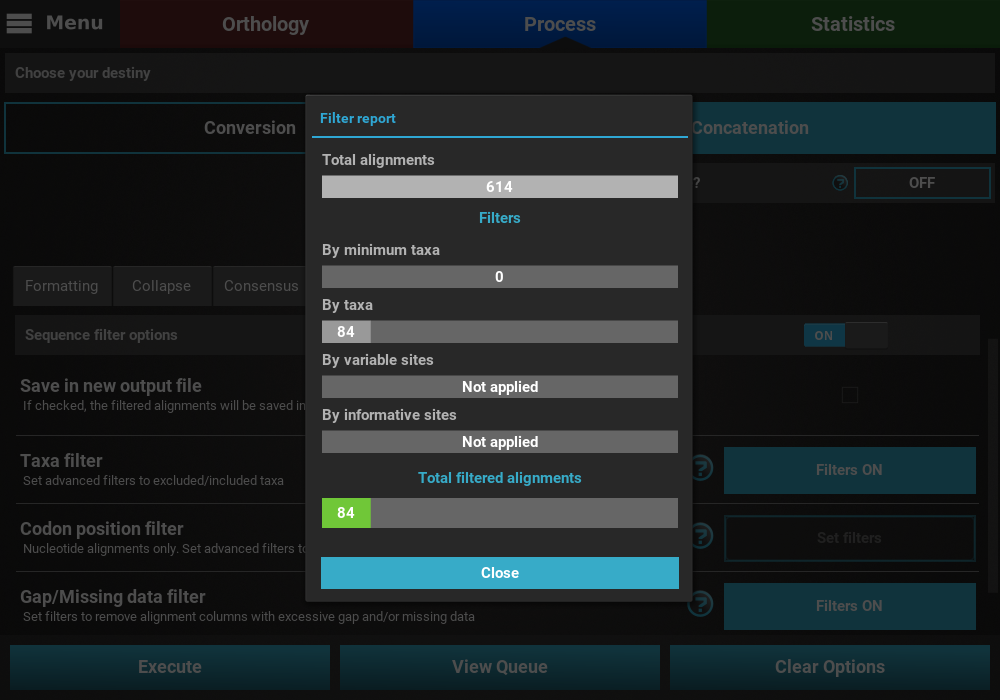
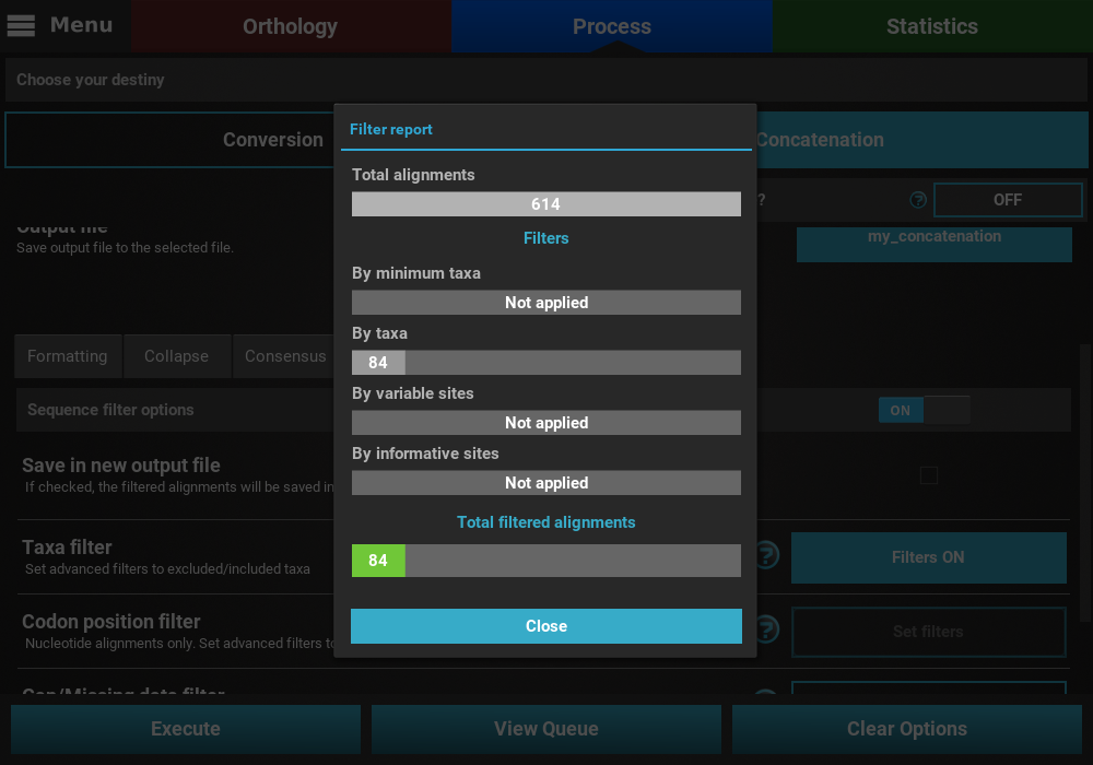
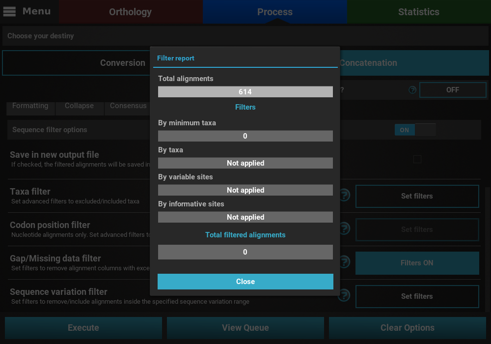
Finally, press the Execute button at the bottom of the Process screen to execute the filter operation. At the end of Filter operations that may remove alignment files from the final output, a Filter report will popup informing how many alignments were filtered. In our case, 84 alignments were filtered (By taxa filter) from the final output.

Codon position filter

Note

This filter is only available for nucleotide alignments.

Turn ON the filter switch to activate the operation. Then click the Set filters button for the Codon position filter option and turn ON the switch on the popup as well.

The Codon position filter operation allows you to remove certain codon positions from the output alignment. Consequently, this option is only available for nucleotide sequences. In many nucleotide alignments it is common to remove the third codon position, as it is generally much more variable and could introduce a substantial amount of phylogenenetic noise. However, this option removes the same codon positions in all input alignments. For example, if you load 10 alignments in TriFusion and exclude the 3rd codon position, you must make sure that all 10 alignments start in the 1st codon position. However, if all alignments start in the 2nd codon position, for instance, removing the 3rd codon position is still possible in TriFusion, by excluding the 2nd positions (which will actually correspond to the 3rd positions in the alignment).

To exclude a given codon position, simply toggle the corresponding button off. Included position button always have a blue background.

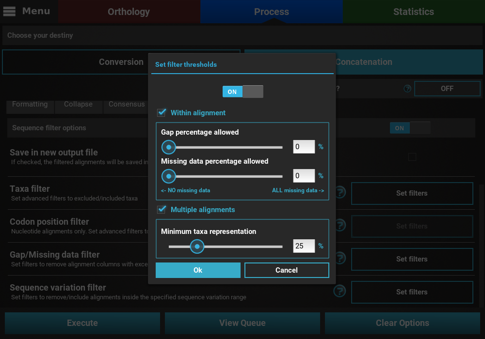
Gap/Missing data filter

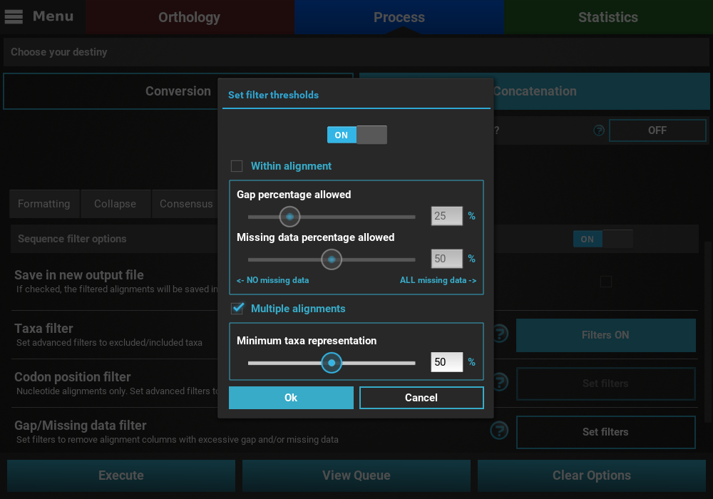
Turn ON the filter switch to activate the operation. Then click the Set filters button for the Gap/Missing data filter option and turn ON the switch on the popup as well.

The Gap/Missing data filter allows user to filter alignment columns (within alignment) and/or alignments (multiple alignments) based on their missing data content. Both filters can be used in combination, if both within alignment and multiple alignments checkboxes are active, or only one of them.

In this example, we will filter both alignment columns and alignment files, so both checkboxes will remain active. Within an alignment, columns can be filtered depending on the amount of gaps or missing data. Gaps refer to the usual gap symbol (“-“) while missing data refers to the sum of gap symbols AND true missing data (“N” for nucleotides or “X” for proteins). These filters provide maximum threshold values in percentages, above which alignment columns are filtered. For example, if the gap percentage allowed option is set to 25% and the missing data percentage allowed option is set to 50%, then alignment columns with more than 25% of gaps OR more than 50% of gaps + true missing data are filtered.

In our case, we are interested in producing an output matrix that contains no missing data, so we will set both sliders to 0%.

Concerning the multiple alignments option, we will be more relaxed. We’ll set the slider to 25%, which means that only alignments with more than 25% of the total data set taxa (12 out of 48 in this case) will be further processed.

When you are happy with the gap/missing data filter settings, click the Ok button. If the Gap/Missing data filter switch was turned ON, the button of the Gap/Missing data filter option should change to Filters ON.

Finally, press the Execute button at the bottom of the Process screen to execute the filter operation. At the end of Filter operations that may remove alignment files from the final output, a Filter report will popup informing how many alignments were filtered. In our case, there were actually no filtered alignments, which means that all input alignments already contained more than 25% of the total taxa.

Sequence variation filter

Turn ON the filter switch to activate the operation. Then click the Set filters button for the Sequence variation filter option and turn ON the switch on the popup as well.

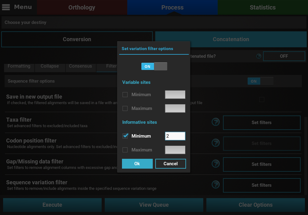
The sequence variation filter allows users to filter alignment files based on the amount of sequence variation. The two supported types of sequence variation are variable sites and informative sites. The different between these types is that variable sites includes all columns with at least one variant, while informative sites only includes variable columns where at least one alternative allele has two or more copies.

Here, you can specify multiple combination of maximum and minimum values for each variation type. When a checkbox is left inactive, it is assumed that there is no boundary for that specific value. For instance, let’s filter our alignments so that only alignments with at least 2 informative sites are processed. To achieve this, check the Minimum box of the informative sites option and set it to 2, but leave the Maximum box unchecked.

If you would like to set an upper limit to the number of informative sites, just check the Maximum box and set a number higher than 2. In this case, let’s put an upper limit of 10 informative sites.

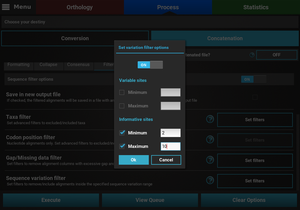
It is also possible to mix both types of sequence variation. For instance, we may want to filter alignments with more than 2 informative sites and less than 200 variable sites.

However, note that certain combination are redundant. For instance, if you set a minimum of informative sites to 2, setting a minimum of variable sites to 1 will have no effect on the final output.

When you are happy with the sequence variation filter settings, click the Ok button. If the Sequence variation filter switch was turned ON, the button of the Sequence variation filter option should change to Filters ON.

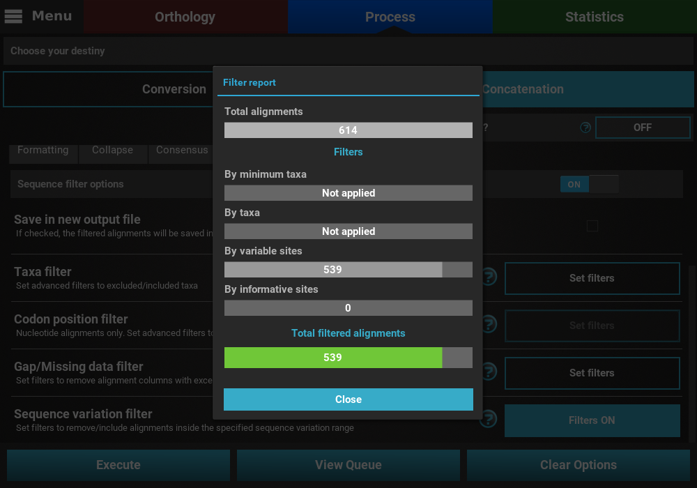
Finally, press the Execute button at the bottom of the Process screen to execute the filter operation. At the end of Filter operations that may remove alignment files from the final output, a Filter report will popup informing how many alignments were filtered. In our case, if we execute filter options of a least 2 informative sites and less than 200 variable sites, a total of 539 alignments will be filtered.

Gap coding

Turn ON the gap coding switch to activate the operation.

The Gap coding operation enables the codification of gaps as a binary matrix that is appended to the final of the alignment matrix. This option is available only when the Nexus format is the only output format selected. Currently, it contains a single available option:

• Save in new output file: This will save the alignment with coded gaps in another output file, separated from the main concatenated/ converted output file. Checking this option will effectively produce two output files - a main output that is only concatenated/converted and another output file with the suffix “_gcoded” that will have the coded gaps. For now, we will not check this option.

The Gap coding method is currently restricted to the one described in Simmons and Ochotenera 2000, however additional methods are expected to be added in future releases.

Combination of three secondary operations

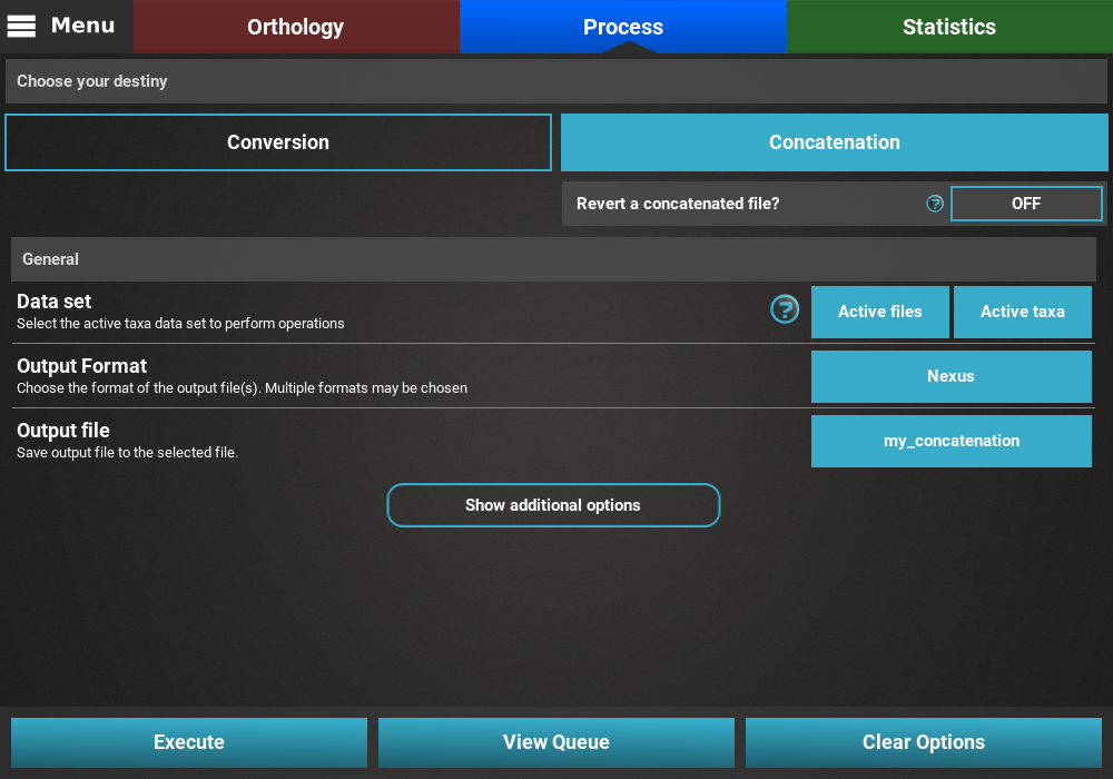
Until now, we only dealt with the activation and usage of individual secondary operations. However, many of these operations can fit rather naturally in combination. Here I’ll demonstrated how a data set of 614 alignments with 48 taxa can be concatenated, collapsed and filtered in a single run, with the condition that the collapsed alignment has to be generated in an independent alignment file.

After loading the data, select the Concatenation main operation in the Process screen. To keep things simple, let’s leave the Data set options in the default values, select only the Nexus output format and provide an output file name (here it will be my_concatenation).

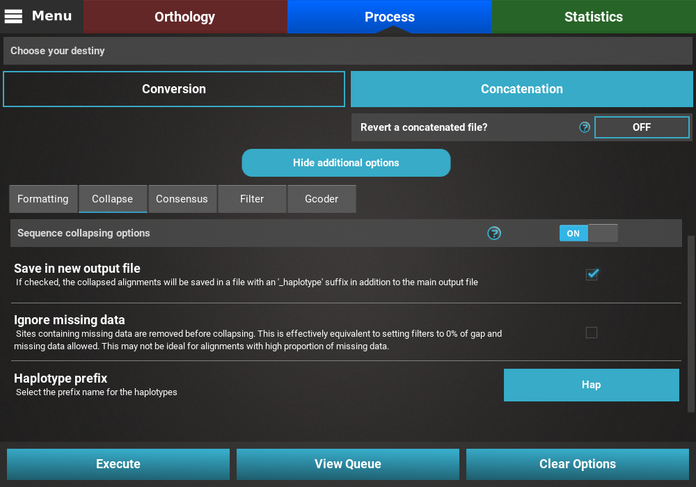
Setting up collapse operation

Open the secondary operations tabbed menu by clicking the Show additional options button, click on the Collapse tab and turn the switch ON.

Since we want to save the collapsed alignment in a separated output that is independent of the remaining operations, we’ll check the Save in new output file box. Our data set contains a fair amount of missing data, so we’ll leave the Ignore missing data box unchecked. Finally, we can leave the haplotype prefix in its default Hap value.

Setting up taxa filter

Here we are interested creating an output data set with alignments that contain any taxon whose name starts with the letter “C”.

Click on the Filter tab and turn the switch ON. Then, click on the Set filters button for the Taxa filter option and activate the switch in the popup. Change the Filter mode to Contain and then click on the Set taxa group button to define the new taxa group.

Let’s manually create a taxa group with all taxa names that start with the letter “C” by clicking the Set manually button.

Once the group has been created, check that the this group is correctly selected in the Taxa filter dialog.

If all checks out, click Ok and the button of the Taxa filter option should now display Filters ON.

Setting up missing data filter

Here we are interested in filtering ONLY alignments that contain less than 50% of the total taxa in the data set. Since we are not interested in the within alignment filtering, let’s uncheck this box and set the Multiple alignments slider to 50%.

Then select the Ok button, and both the Taxa filter and Gap/Missing data filter buttons should now display Filters ON.

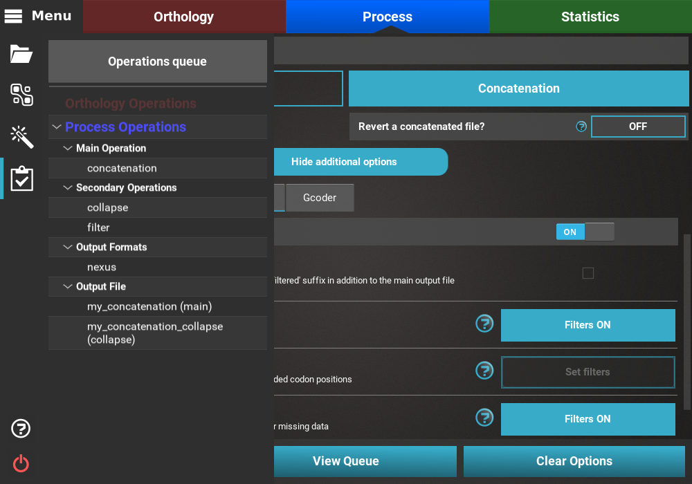
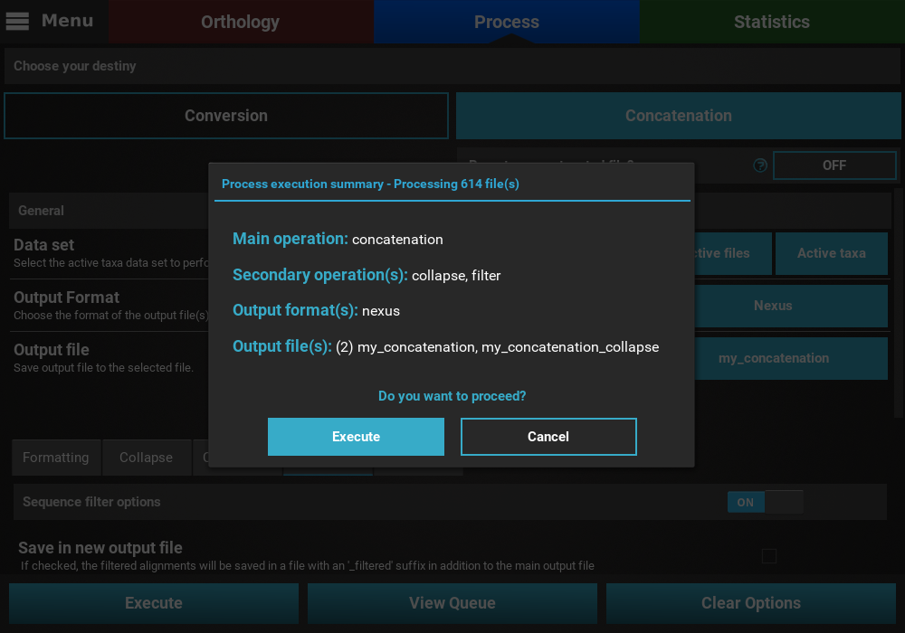
Checking selected options

All currently active options can be viewed by clicking the View Queue button at the bottom of the Process screen. This will open the Menu side panel and show that:

• The main operation is Concatenation;
• There are two active secondary operations: Collapse and Filter;
• The Nexus output format is the only selected;
• There are two expected output files: The main output, my_concatenation, and the separate output file that will only contain the result of the concatenation and collapse operations, my_concatenation_collapse.

Execution

If everything checks out, click the Execution button at the bottom of the Process screen to show the small popup that displays a summary of the process execution and then click the Execute button to begin the execution.

At the end of the execution, a filter report will appear showing the number of alignments that were filtered by the active filters. Since we only activated two of the four filters that can remove alignments from the final output, the values for the other two filters display a Not applied message. For the active filters, the number of alignments removed due to that filter is displayed. In this case, no alignment was removed from the Gap/Missing data filter (it seems all alignments already contained more than 50% of the total taxa) and 84 alignments were removed by the Taxa filter.