Basic conversion/concatenation
Note
Data availability for this tutorial: the medium sized data set of 614 genes and 48 taxa that will be used can be downloaded here.
Which input alignments can be used?
TriFusion was designed to impose as little limitations when loading alignment data as possible. All of the supported input formats and sequence types can be provided simultaneously to TriFusion. If you have nucleotide and protein sequence alignments in multiple formats, such as fasta, nexus, phylip, etc, you can load them simultaneously and all of the relevant information will be automatically detected.
When using the Concatenation operation, and if you are interested in generating the partitions definition in Nexus or Phylip formats, TriFusion will handle the partition ranges for you. If a mixture of nucleotide and protein alignments is loaded, the nucleotide and amino acid residue ranges will be sorted by sequence type, updating the partition ranges and generating the correct Nexus header.
The bottom line is that regardless of the type and format in which you have your data, it should be fine to load it into the application and TriFusion will deal with all the details automatically.
Load alignments
As already covered in a separate tutorial (see Load data into TriFusion), alignment data can be loaded into TriFusion in three different ways. Here we will use the file browser to load an entire directory where 614 alignments files are stored.
Navigate to Menu > Open/View Data and click the Open file(s) button.
This will open the main file browser.
The input data type is already correctly set to Alignment/Sequence set,
so we’ll leave that as it is. Then, navigate the file browser until you
find the directory containing the alignment files. In this case, all
alignments are stored in a directory named Version2. Since TriFusion
supports the selection of directories (in which case all files inside the
specified directory will be loaded), I will only select the Version2
directory and click Load & go back button. At the end of the data
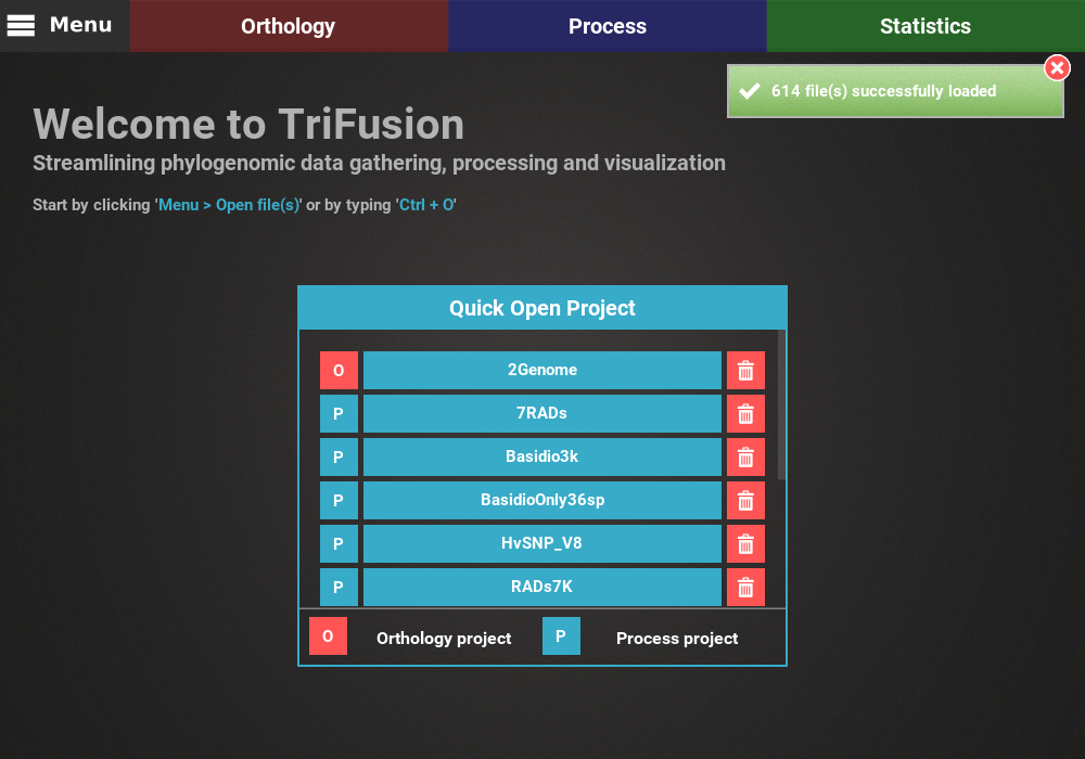
loading, a popup informs how many files were loaded.
Note
If you know that not all files in the selected directory are alignments, you could still load that particular directory. All invalid alignment files will be ignored when the data is loaded.
Conversion/concatenation
The Conversion and Concatenation options are found in the
Proces screen. In this screen, select either Conversion or
Concatenation to reveal the General options, which are mostly
the same for both operations.
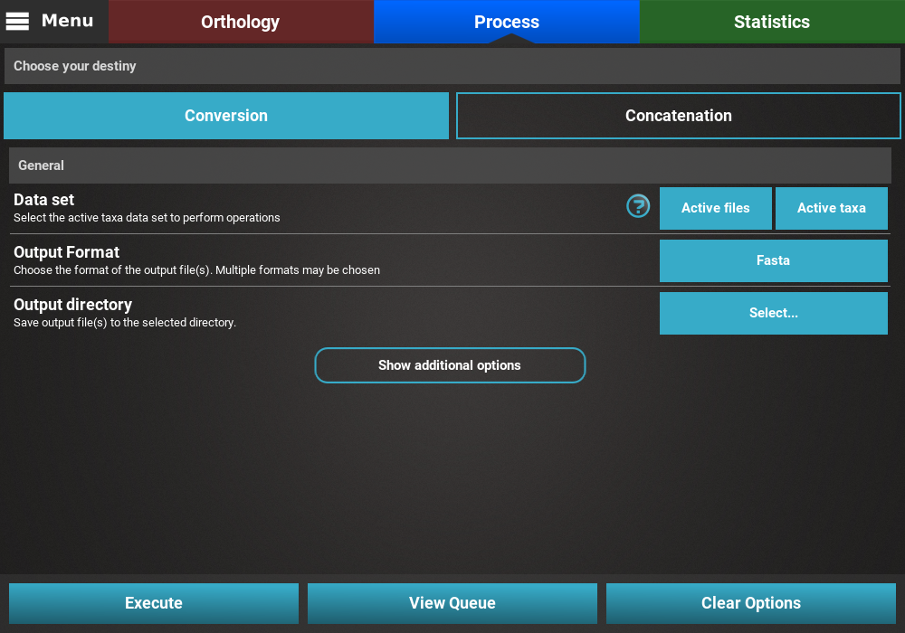
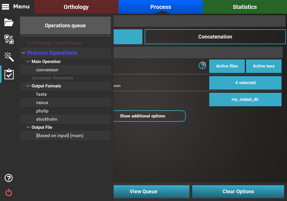
General options
The first option, Data set, specifies which active data set will be used for the conversion operation (see Data set groups tutorial or Concatenation with custom active data sets below). For now we’ll leave it in the default value.
In the second option, Output format, you can choose one or more output formats to convert the input data. In this case we will choose 4 output formats (fasta, phylip, nexus and stockholm). Some output formats also contains specific additional options that can be viewed by clicking the corresponding settings button. Also note that some formats can only be used with the concatenation operation.

THe final general option is used to specify where you want to generate the output alignment(s).
In the case of Conversion, the Output directory option is used to select the directory where the output files will be generated. Here, the name of each output file will be based on the corresponding input file (for instance, the input alignment.fas will be converted into alignment.nex when the Nexus output format is specified). However, you can specify a suffix that will be appended to the end of every output file in the Suffix text box. For example, specifying “_variant1” as the suffix will create output files like alignment1_variant1.nex.
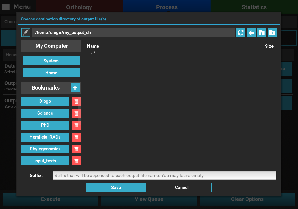
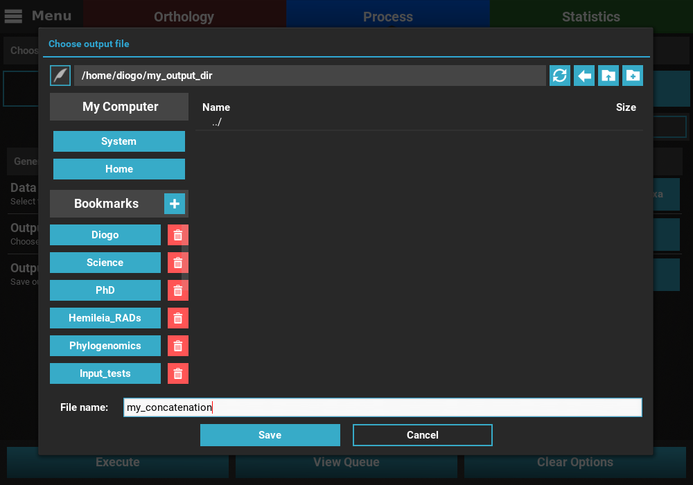
In the case of Concatenation, the Output file option is used to specify the directory AND name of the output file. For example, we could name our concatenated output file “my_concatenation”. The extension is automatically added.
After setting up these general options, you can click the View Queue
button at the bottom of the screen to get an overview of the selected
options. There you’ll see that the 614 files are set to be converted
into 4 output formats in a number of output formats whose name will be
based on the input.
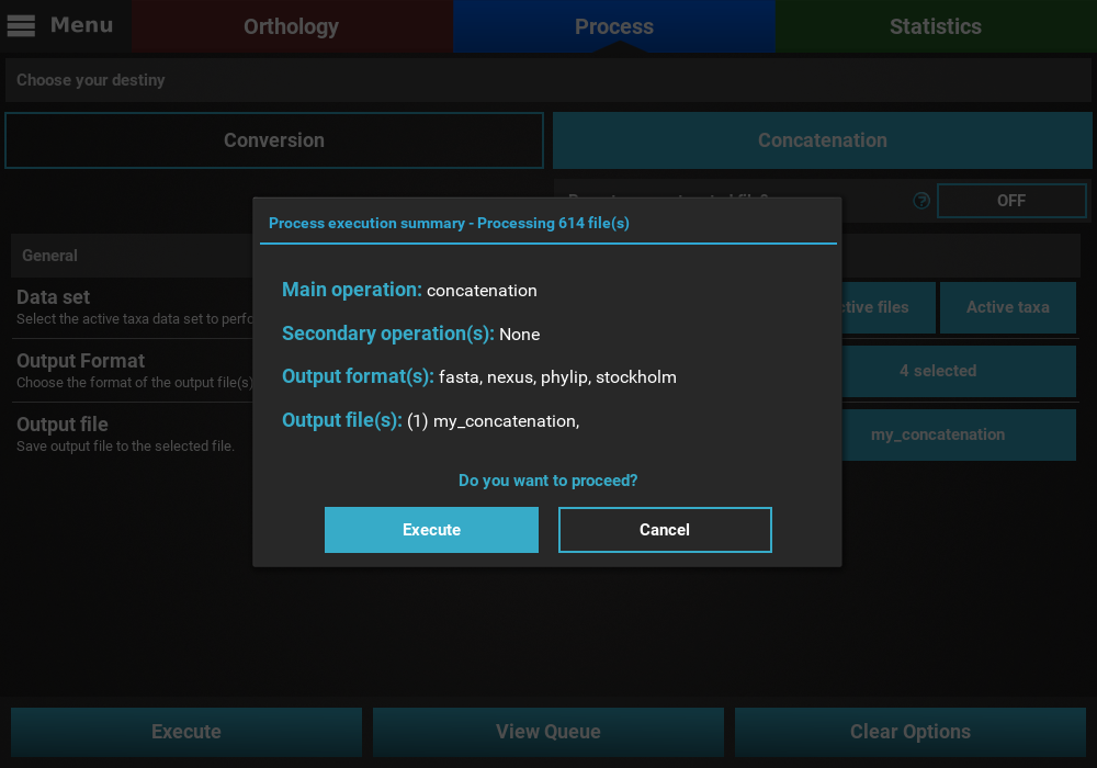
Execution
The execution of either Conversion or Concatenation operations is
started by clicking the Execute button at the bottom of the screen.
This will open an execution summary with information on the selected main
operation, the selected secondary operations (if any), the selected
output formats and the expected number of output files. In the case of
Concatenation the actual output file name should appear.
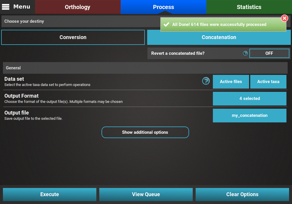
If you’re happy with these settings, click the Execute button, and
the Conversion/Concatenation operation will be carried out. At the
end of the execution, an informative popup should appear with a
notification that all files were successfully processed.
Concatenation with custom active data sets
Note
Operations on custom data sets can also be applied with the Conversion operation. In this case, however, it just means that the alignments and taxa that are not converted.
In many cases, additional operations may be desired on specific subsets of the total loaded dataset. Here we’ll see one way of performing an additional concatenation operation on a custom made data set. More information is available in the Data set groups tutorial.
Creating and changing the active data set
Suppose we were interested in concatenating the same 614 files, but only for taxa whose names start with the letter “A”. And after that for taxa whose names start with the letter “C”. Since I need to create two taxa groups (say, A_taxa and C_taxa), we will also explore two methods of creating these data sets.
Using the side panel toggling method
To create an active data set that contains, for example, only taxa whose
names start with an “A”, go to Menu > Open/View Data and selected the
Taxa tab. There are three taxa whose name starts with an “A”.
The quickest way to selected only these taxa would be to click the
Deselect All button and then toggling ON the desired three taxa.
Using the data set creation dialog
To create the C_taxa via the data set creation dialog, go to
Menu > Dataset Groups, click the Taxa tab, and then the
Set new taxa group button. Since we’re dealing with a small number of
taxa, we will set the taxa group manually in TriFusion. In the
taxa group creation dialog, select the taxa with names starting with
a “C” (here using Shift + clicking to selected the seven taxa is
convenient), specify the group name and click OK.

Execution with custom active data sets
We’ll start with the execution of the Concatenation of the 614 files
for the A_taxa taxa group. We need to make sure that the value of the
Data set general option is set to Active taxa, so that TriFusion
will use the three active taxa previously defined. Then, click
Execute and complete the concatenation operation as before.
Now for the C_taxa group, select the name of this group in the drop down menu of the Data set general option.
Once the C_taxa group is selected, click the Execute button and
complete the concatenation as before.
Concatenation with custom partitions
One of the convenient features of TriFusion is that it allows you to easily edit or import from a text file the partitions of your current data set. You don’t really have to worry about the range, order, size of the partitions, as long as you don’t mix partitions of different sequences types (e.g. protein and nucleotide). You can also specify some substitution models for your partitions for output formats that support that kind of information (Nexus and Phylip). You can check the more detailed Partitions and substitution models tutorial.
Load data
Here we’ll see how the concatenation operation can seamlessly deal with any partition scheme you provide, with or without information on the substitution model. For this part of the tutorial we’ll use a smaller data set of 10 alignments so that it is easier to follow the changes. Nevertheless, TriFusion is able to deal with thousands of partitions as easily.
This is a mixed data set containing Fasta and Phylip alignments of protein and nucleotide sequences. Let’s import the data using the drag and drop method.

If you navigate to Menu -> Open/View Data and click on the Partitions
tab you can see that TriFusion attributes a partition to each individual
input file by default (unless partition schemes are provided when loading
Nexus files).

Basic concatenation
Loading a mixed data set (nucleotide and protein sequences) raises the immediate issue that, in formats such as Nexus, the ranges of the nucleotide and protein sequences has to be defined in the header, in addition to the partitions definition. TriFusion does this for you and simplifies the issue by grouping nucleotide and protein files/partitions together, regardless of their input order.
First, let’s perform a Concatenation operation without further
modification of the default partitions. Specify the Nexus as the output
format, provide an output file and click Execute.
If you inspect the output Nexus file, you can see that the header now has the information on the mixed data set:
#NEXUS
Begin data;
    dimensions ntax=49 nchar=6134 ;
    format datatype=mixed(dna:1-2790,protein:2791-6134) interleave=no gap=-;
With the concatenated alignment having the first 2790 characters as nucleotides and the remaining as amino acid residues. At the end of the file, the partitions are also correctly defined and ready for downstream software like MrBayes:
begin mrbayes;
    charset BasidioOnly2585dnaphy = 1-1458;
    charset BasidioOnly2685dnaphy = 1459-1722;
    charset BasidioOnly2686dnaphy = 1723-2259;
    charset BasidioOnly2687dnaphy = 2260-2790;
    charset BasidioOnly2585proteinfas = 2791-3837;
    charset BasidioOnly2685proteinfas = 3838-3959;
    charset BasidioOnly2686proteinfas = 3960-4153;
    charset BasidioOnly2687proteinfas = 4154-4373;
    charset BasidioOnly2689proteinfas = 4374-5178;
    charset BasidioOnly2690proteinfas = 5179-6134;
    partition part = 10: BasidioOnly2585dnaphy, BasidioOnly2685dnaphy, BasidioOnly2686dnaphy, BasidioOnly2687dnaphy, BasidioOnly2585proteinfas, BasidioOnly2685proteinfas, BasidioOnly2686proteinfas, BasidioOnly2687proteinfas, BasidioOnly2689proteinfas, BasidioOnly2690proteinfas;
    set partition=part;
end;
Merge partitions
Partitions can be merged in any number and order, provided that they share the same sequence type (nucleotide partitions can only be merged with nucleotide). We can, for instance, merge all protein partitions together and the first and last nucleotide partitions. To accomplish this, select all partitions you wish to merge and click the merge partitions button at the bottom of the panel.

When we repeat the Concatenation operation, we can see that the Nexus header remains the same, but the partitions have been updated. Notice that even though we merged non-contiguous partitions, they appear with the same range. This is because TriFusion will first sort the partition sequences so that they become contiguous and only then it will write the output file:
begin mrbayes;
    charset nuc1 = 1-1989;
    charset BasidioOnly2685dnaphy = 1990-2253;
    charset BasidioOnly2686dnaphy = 2254-2790;
    charset proteinparts = 2791-6134;
    partition part = 4: nuc1, BasidioOnly2685dnaphy, BasidioOnly2686dnaphy, proteinparts;
    set partition=part;
end;