Partitions and substitution models
Note
Data availability for this tutorial: a small concatenated alignment with the corresponding partition files is available here.
TriFusions offers several features to import and handle partitions and substitution models for alignment files. Here I’ll describe some of the most common operations.
How to import partitions
From the alignment file
Note
This is only supported for Nexus input files.
Nexus alignment files often have a charset block after the alignment matrix where its partitions are described:
# NEXUS
Begin data; dimensions ntax=20 nchar=425 ;
format datatype=DNA interleave=no gap=- missing=n ;
matrix

(... alignment matrix...)

;
end;
begin mrbayes;
charset Teste1 = 1-85;
charset Teste2 = 86-170;
charset Teste3 = 171-255;
charset Teste4 = 256-340;
charset Teste5 = 341-425;
partition part = 5: Teste1, Teste2, Teste3, Teste4, Teste5;
set partition=part;
end;
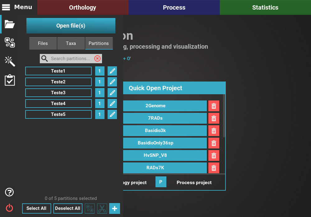
In this case, 5 partitions were defined using the charset keywords. When this file is loaded into TriFusion, this block is used to define the partitions in the Partitions tab of TriFusion’s side panel.
From a partitions file
TriFusion can import partitions schemes formatted in one of two popular formats. Here I’ll exemplify how partitions can be imported in either case after loading a concatenated file of 5 alignments into TriFusion, named concatenated_file.fas.
Nexus charset block
A Nexus partitions file is a simple text file containing the charset block defining the partitions for an alignment file. In our case, the partition file (named concatenated_file.nxpart) would look something like this:
# charset [name of partitions] = [partition-range];
charset Teste1.fas = 1-85;
charset Teste2.fas = 86-170;
charset Teste3.fas = 171-255;
charset Teste4.fas = 256-340;
charset Teste5.fas = 341-425;
RAxML partition file
This is the partition file usually required by RAxML for partitioned alignments. Here, partitions are simply defined in each line by providing the substitution model (optional), the name of the partition and then its range. We’ll name this file concatenated_file.partFile:
GTR, BaseConc1.fas = 1-85
GTR, BaseConc2.fas = 86-170
GTR, BaseConc3.fas = 171-255
GTR, BaseConc4.fas = 256-340
GTR, BaseConc5.fas = 341-425
Importing the partition file
To import this partition scheme, and assuming that our concatenated_file.fas
is already loaded into TriFusion, navigate to Menu > Open/View Data and
click the Partitions tab.
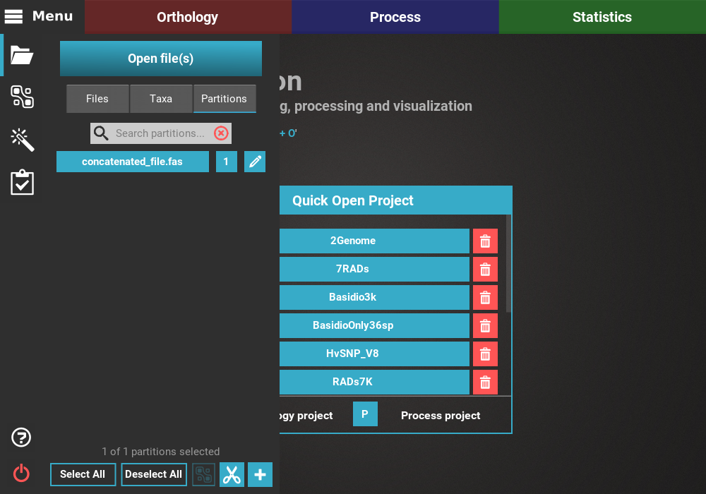
There is already a single partition defined because TriFusion always
attributes one partition for each input alignment by default.
However, by providing a partition scheme, any previously defined partitions
will be discarded. The partition scheme can be provided by clicking
the + button at the bottom of the panel and selecting the partition file
in the file browser. You can try to import either the Nexus or RAxML
partitions file, since the result will be the same.
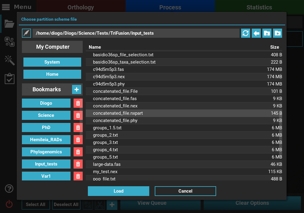
After selecting the partition file, TriFusion will perform several checks to ensure the consistency of the partitions according to the alignment file. If all checks out, the 5 defined partitions will appear in the Partitions tab.
How to create/split partitions
Let’s assume we still have the concatenated_file.fas without defined
partitions loaded into TriFusion. To create/split partitions,
navigate to Menu > Open/View Data and click on the Partitions tab.
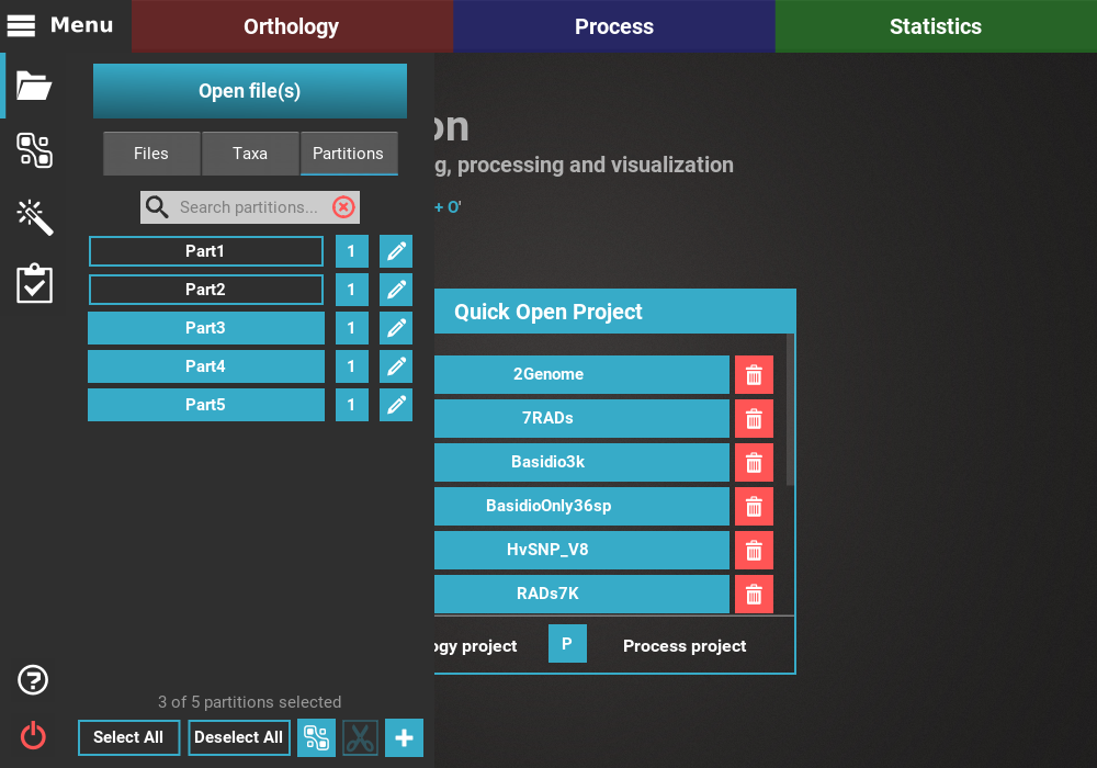
By default, TriFusion creates a single partition for each input alignment file. This means that when a new partition is created, it is actually split from an existing partition. In this way, we can re-create the 5 partitions that were defined in the sections above. However, as you will see, this taks is more suitable for small punctual modification to the partition scheme than to define partitions from scratch. For larger partitions schemes, using partition files is always easier and more convenient.
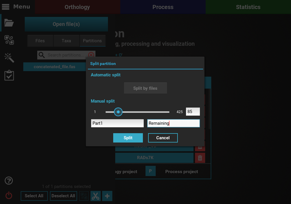
To create the first partition, which should have the range from position 1 to 85, select the concatenated_file.fas partition button. When you do, the Scissor button at the bottom of the panel should become available.
When you click it, a dialog will allow you to split the selected partition
into two. You can use the slide or the text input to define the range
of the first partition. Let’s name this partitions Part1 and provide
a temporary Remaining name for the remaining range. Then, click Split.
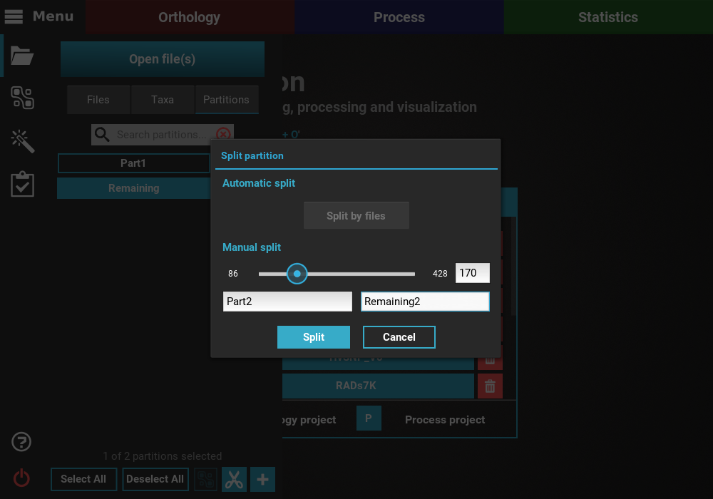
As you can see, the new partition Part1 was created. We can continue this process of creating 85bp partitions, by clicking the Remaining partition button, and then the Scissors icon to define a new partition.
Now, the Remaining partition will start at the 86th bp, so we’ll need to add the length of the second partition.
How to merge pre-existing partitions
Partitions in TriFusion cannot be actually removed, since any part of the alignment must be covered by one partition. However, partitions can be merged to produce a similar effect. For instance, if we load the concatenated_file.nex file into TriFusion, it will automatically set 5 partitions for this alignment.
If you want to remove, say, the last two partitions, you can merge them
with the last standing partition. Click on the partition buttons
Part3, Part4 and Part5 and the Merge button at the end of the
panel should become available.
Clicking the Merge button will ask you for the name of the
new partition. We’ll name it end_partition.
This will effectively remove the last two partitions, and append their range to the previouus Part3 partition. The merge procedure can be combined with the split procedure to fine tune partition ranges.
Ultimately, you can “remove” all partitions by merging all partitions
in a single one. For this, simply select all partitions and click
the Merge button.
Non-contiguous partitions
There is no requirement for partitions to be contiguous before merging. The only limitation when merging partition is that they must be of the same sequence type (nucleotide or protein).
If we want, we could merge the first and last partitions in a new partition named extremes.

By merging non-contiguous partitions together, TriFusion will automatically merge the sequence data into continuous segments and the remaining partition ranges. Therefore, if you perform a Concatenation into a Nexus output format, you’ll see that the sequence data from the last alignment will now appear merged with the sequence from the first alignment. Indeed, the order of the new merged partition is based on the starting position of the first selected partition.
As an example, the result of the concatenated nexus file of this merger will be:
begin mrbayes;
    charset extremes = 1-170;
    charset Teste2 = 171-255;
    charset Teste3 = 256-340;
    charset Teste4 = 341-425;
    partition part = 4: extremes, Teste2, Teste3, Teste4;
    set partition=part;
end;
Change the partition’s name
Partition names can be easily changed in TriFusion. Navigate to
Menu > Open/View Data and click on the Partitions tab.
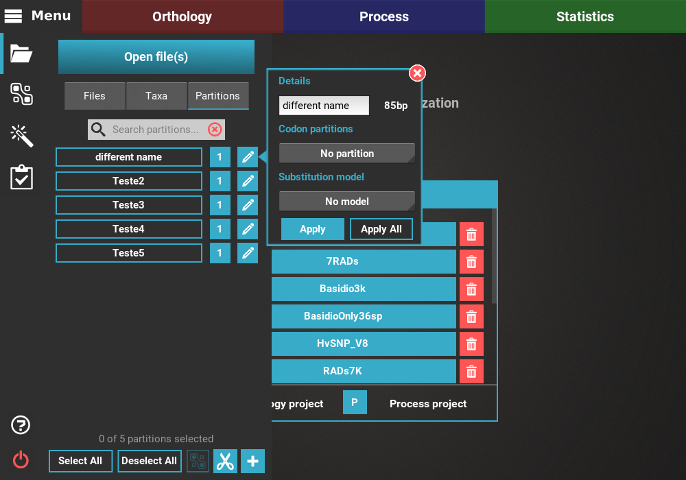
To change the name of one partition, say Test1, click on the corresponding Pencil button. The current name should appear in a text field under the Details section.

Then, modify the name no your liking and press Enter to change it.
Edit the substitution model
TriFusion supports the specification of substitution models and codon partitions. However, note that this information is can only be included in Nexus output formats or in the RAxML partition file that is generated for the Phylip output format.
To set/change the substitution model and/or codon partitions of a
partition, navigate to Menu > Open/View Data and click on the
Partitions tab.
Then, click on the Pencil button of any partition to open the edition dialog.

You can choose a codon partition scheme using the drop down menu under the Codon partitions section. All possible codon partition schemes are listed, included the option to have no sub-partitions. In this example, lets create separate partitions for each codon position by selecting the 1 + 2 + 3 value.
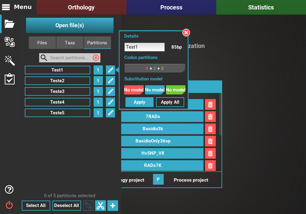
Then, you can choose the appropriate model for each partition, following the color code. For example, we want to set JC for the first codon (red), HKY for the second codon (blue) and GTR for the third codon (green).

If you want to make the change only for the current partition, click
the Apply button. If you want to make this change for all partitions,
click the Apply All button.
If we apply this codon partition and substitution models to all partitions, the final result in a concatenated Nexus file will have the partitions defined using the notation for codon partitions:
begin mrbayes;
    charset Teste1_1 = 1-85\3;
    charset Teste1_2 = 2-85\3;
    charset Teste1_3 = 3-85\3;
    charset Teste2_86 = 86-170\3;
    charset Teste2_87 = 87-170\3;
    charset Teste2_88 = 88-170\3;
    charset Teste3_171 = 171-255\3;
    charset Teste3_172 = 172-255\3;
    charset Teste3_173 = 173-255\3;
    charset Teste4_256 = 256-340\3;
    charset Teste4_257 = 257-340\3;
    charset Teste4_258 = 258-340\3;
    charset Teste5_341 = 341-425\3;
    charset Teste5_342 = 342-425\3;
    charset Teste5_343 = 343-425\3;
    partition part = 15: Teste1_1, Teste1_2, Teste1_3, Teste2_86, Teste2_87, Teste2_88, Teste3_171, Teste3_172, Teste3_173, Teste4_256, Teste4_257, Teste4_258, Teste5_341, Teste5_342, Teste5_343;
    set partition=part;
end;
Below the partitions block, the substitution models were also specified for each partition:
begin mrbayes;
lset applyto=(1) nst=1;
prset applyto=(1) statefreqpr=fixed(equal);
lset applyto=(2) nst=2;
prset applyto=(2) statefreqpr=dirichlet(1,1,1,1);
lset applyto=(3) nst=6;
prset applyto=(3) statefreqpr=dirichlet(1,1,1,1);
lset applyto=(4) nst=1;
prset applyto=(4) statefreqpr=fixed(equal);
lset applyto=(5) nst=2;
prset applyto=(5) statefreqpr=dirichlet(1,1,1,1);
lset applyto=(6) nst=6;
prset applyto=(6) statefreqpr=dirichlet(1,1,1,1);
lset applyto=(7) nst=1;
prset applyto=(7) statefreqpr=fixed(equal);
lset applyto=(8) nst=2;
prset applyto=(8) statefreqpr=dirichlet(1,1,1,1);
lset applyto=(9) nst=6;
prset applyto=(9) statefreqpr=dirichlet(1,1,1,1);
lset applyto=(10) nst=1;
prset applyto=(10) statefreqpr=fixed(equal);
lset applyto=(11) nst=2;
prset applyto=(11) statefreqpr=dirichlet(1,1,1,1);
lset applyto=(12) nst=6;
prset applyto=(12) statefreqpr=dirichlet(1,1,1,1);
lset applyto=(13) nst=1;
prset applyto=(13) statefreqpr=fixed(equal);
lset applyto=(14) nst=2;
prset applyto=(14) statefreqpr=dirichlet(1,1,1,1);
lset applyto=(15) nst=6;
prset applyto=(15) statefreqpr=dirichlet(1,1,1,1);
unlink statefreq=(all) revmat=(all) shape=(all) pinvar=(all) tratio=(all);
end;
Note that all codon partitions have unlinked models. However, you can also link codon models in TriFusion. For instance, we could choose the codon partition option of (1 + 2) + 3 to link the same substitution model of the first two codons and keep a different one for the third codon. Let’s set the HKY model for the first two codons and the GTR for the third.

If we repeat the concatenation to a Nexus output file, you can see that the while the partition block is the same, the definition of the substitution models has changed:
begin mrbayes;
lset applyto=(1) nst=2;
prset applyto=(1) statefreqpr=dirichlet(1,1,1,1);
lset applyto=(2) nst=2;
prset applyto=(2) statefreqpr=dirichlet(1,1,1,1);
lset applyto=(3) nst=6;
prset applyto=(3) statefreqpr=dirichlet(1,1,1,1);
lset applyto=(4) nst=2;
prset applyto=(4) statefreqpr=dirichlet(1,1,1,1);
lset applyto=(5) nst=2;
prset applyto=(5) statefreqpr=dirichlet(1,1,1,1);
lset applyto=(6) nst=6;
prset applyto=(6) statefreqpr=dirichlet(1,1,1,1);
lset applyto=(7) nst=2;
prset applyto=(7) statefreqpr=dirichlet(1,1,1,1);
lset applyto=(8) nst=2;
prset applyto=(8) statefreqpr=dirichlet(1,1,1,1);
lset applyto=(9) nst=6;
prset applyto=(9) statefreqpr=dirichlet(1,1,1,1);
lset applyto=(10) nst=2;
prset applyto=(10) statefreqpr=dirichlet(1,1,1,1);
lset applyto=(11) nst=2;
prset applyto=(11) statefreqpr=dirichlet(1,1,1,1);
lset applyto=(12) nst=6;
prset applyto=(12) statefreqpr=dirichlet(1,1,1,1);
lset applyto=(13) nst=2;
prset applyto=(13) statefreqpr=dirichlet(1,1,1,1);
lset applyto=(14) nst=2;
prset applyto=(14) statefreqpr=dirichlet(1,1,1,1);
lset applyto=(15) nst=6;
prset applyto=(15) statefreqpr=dirichlet(1,1,1,1);
unlink statefreq=(all) revmat=(all) shape=(all) pinvar=(all) tratio=(all);
link statefreq=(1,2) revmat=(1,2) shape=(1,2) pinvar=(1,2) tratio=(1,2);
link statefreq=(4,5) revmat=(4,5) shape=(4,5) pinvar=(4,5) tratio=(4,5);
link statefreq=(7,8) revmat=(7,8) shape=(7,8) pinvar=(7,8) tratio=(7,8);
link statefreq=(10,11) revmat=(10,11) shape=(10,11) pinvar=(10,11) tratio=(10,11);
link statefreq=(13,14) revmat=(13,14) shape=(13,14) pinvar=(13,14) tratio=(13,14);
end;
At the end of this block, the substitution parameters for all first and second codons were linked.